CO2 removal system analytics

CO2 REMOVAL

CO2 removal system analytics

Arun Murugan and Mike Antony of FITIRI and Venkat Pattabathula of SVP Chemical Plant Services discuss the COORS Analytics system for more accurate prediction of the performance of a CO 2 removal system.

The level of CO2 in the atmosphere is now over 410 ppm, yet when the authors were in chemical engineering classes in late 1970s, we used a value of 330 ppm. Such an increase by human activities in so short a span of time and the consequent weather calamities of recent years has pushed humanity to think about this existential threat. Any technology which can remove CO 2 from the atmosphere or industrial waste gas or flue gas streams will thus be one of the most critical technologies in the years ahead. Furthermore, CO 2 removal systems play a critical role in industrial chemical production such as the manufacturing of ammonia, hydrogen, LNG and in natural gas purification plants.

CO2 removal systems are designed and their performance predicted using chemical engineering techniques such as McCabe and Thiele diagrams and other analytical models. But actual performance of the system varies from plant to plant even with the same design. We call this a ‘personality trait’ for CO 2 systems – no two plants behave the same way, due to too many design and operating variables. It is simply impossible to correlate the performance to engineering equations and analytical models. A CO2 removal system with its own ‘personality’ is thus an ideal engineering problem for data analytics and artificial intelligence.

COORS Analytics stands for CO2 (COO) Removal System Analytics. With COORS, we can accurately predict the performance of a system when operating parameters are changed, and we can predict optimum operating parameters for a new or modified plant.

CO 2 removal processes

There are number of technologies available for CO2 removal using both physical and chemical solvents. The amine-based solvent aMDEA has emerged as the leader among all technologies based on ease of operation, control of corrosion and overall energy consumption. Different technologies used in CO2 removal systems mainly vary in the solvent used. Hot potash systems, Catacarb, Vetrocoke, Selexsol, Rectisol, GV Vetrocoke, MEA, DME, aMDEA, Sulfinol, propylene carbonate etc are some of the most popular in the industry. In almost all systems, CO2 is first absorbed in a solution in an absorption tower with trays or packed beds at high pressure and low temperature, and then the solution is recovered by stripping in a regeneration tower at low pressure and high temperature.

Some of the various removal processes are as follows:

1. Water scrubbing: The oldest method, water scrubbing, is practically abandoned in many plants. The CO2 is absorbed in water under pressure and the water is regenerated by a release in pressure. Most of the energy contained in the high pressure water is recovered by a hydraulic turbine which, along with an electric motor, drive the high pressure water pump. Although this method is simple and inexpensive, hydrogen is dissolved along with the CO2 and therefore the H2 loss is appreciable, amounting to 1.52.5% when the scrubber is operated at 7.2 bar. Several schemes were proposed for recovering hydrogen, but this required additional equipment and increased investment that couldn’t be justified via the value of the hydrogen recovered.

2. MEA absorption: The first generation of single-train plants often used a monoethanolamine (MEA) solution with a high demand of low-grade heat for solvent regeneration. With corrosion inhibition systems, the amine strength could be raised and solvent circulation reduced, saving heat and mechanical energy.

3. Selexol: This process uses polyethylene glycol dimethyl ether as a solvent, which is stable, non-corrosive, not very volatile, but has a rather high capacity to absorb water. For this reason, a relatively dry gas is required, which is achieved by chilling.

4. Rectisol: This process seems to be the prime choice in partial oxidation plants, and is very versatile and allows a number of different configurations.

5. Sulfinol: The Sulfinol process uses a mixture of sulpholane and di-isopropanolamine (DIPA). The Sulfinol solution is replaced by others due to the high cost of solvent loss and usage of heavy metals as corrosion inhibitors.

6. Hot potash systems: Commercial hot potash systems differ in the type of activator used to increase the reaction rate between the CO2 and the solvent. The activators enhance mass transfer and thus influence not only the regeneration energy demand but also the equipment sizing. The various hot potassium solvents are as follows:

• The Catacarb process, with amine and borate as the activator.
• The Giammarco-Vetrocoke process with glycine and various ethanolamines as the activators.
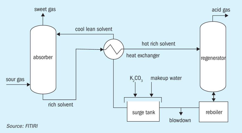
• The Benfield Loheat process with DEA as the activator. Many variations in the flow sheet are operating in different applications. A simplified flow diagram of the Benfield process is shown in Figure 1.

Benfield technology uses hot potassium carbonate as the absorbent. There are hundreds of installations of Benfield systems around the world. When CO2 is absorbed, the carbonate is converted to bicarbonate and therefore this system is a chemical absorption. The Benfield system offers very stable operation, but the solution loaded with CO2 is very corrosive and therefore needs a corrosion inhibitor. Benfield uses pentavalent vanadium (V5+ ) as a corrosion inhibitor, and when it undergoes the corrosion inhibition reaction it is reduced to tetravalent vanadium (V4+ ). The solution also uses DEA as the promoter.

Fig. 1: Benfield basic process schematic

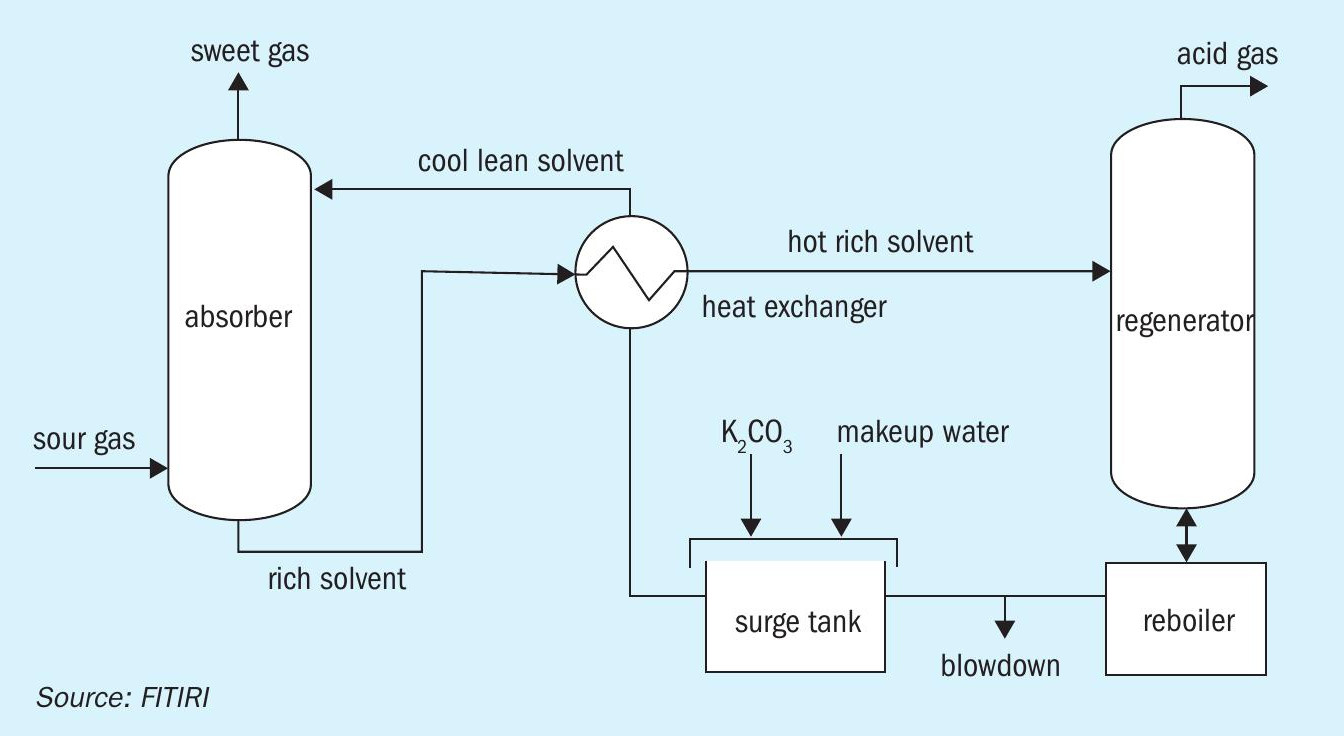
The process contains a gas absorption step and a carbonate regeneration step. Potassium carbonate (K2 CO3 ) is the alkali in the absorption solvent. K2 CO3 reacts with CO2 and H2 S in the absorber tower, forming bicarbonate (HCO3 ) and bisulphide (HS-1 ). This reaction enables the solvent to dissolve significantly more CO2 and H2 S than is possible with pure water. This rich solvent is then steam stripped of the absorbed CO2 and H2 S in the regeneration tower. The regenerated solvent is recycled back to the absorber after energy recovery using heat exchangers.

7. aMDEA: A leading process today is the BASF’s activated methyl diethanolamine (aMDEA) with a special activator. Because of the low vapor pressure of aMDEA, the solvent losses are at a minimum. The CO2 binds much less strongly to MDEA than to MEA and hence requires less energy for regeneration. Many MEA solvent systems were revamped by swapping the solvent without a need to change the process equipment.

Case study

The plant chosen for the study was Incitec Pivot Ltd’s (IPL) Gibson Island ammonia plant (part of a larger fertilizer complex) in Brisbane, Australia. The plants at this site produce ammonia, urea, granular ammonium sulphate, and liquid CO2 . The Gibson Island Product Distribution Centre dispatches approximately 550,000 t/a of fertilizers to IPL customers. The site also has a 160 t/d liquid carbon dioxide plant that supplies half the liquid CO2 in Queensland, and is the main source of CO2 in carbonated soft drinks in Queensland and northern New South Wales.

CO2 removal at Gibson Island

The IPL Gibson Island plant uses the BASF aMDEA process, which offers energy efficient and reliable operation using an activated MDEA solvent for CO2 absorption. The activator accelerates the rate of CO2 absorption and is considered to be a quasi-physical absorption system.

Though COORS analytics can predict the performance of different related flow sheets under aMDEA system, we use a more popular flow diagram with lean and rich solutions, one stage flash, process and steam reboilers and regenerator overhead condenser and reflux systems.

Process gas exiting the low temperature shift converter (LTS) is first cooled to just above its dew point using the LTS outlet desuperheater, DSHT602. The gas then passes through the aMDEA reboilers, E602A and E602B. Here heat is transferred to the aMDEA solution and most of the steam in the process gas condenses as the temperature drops. The mixture of process gas and water then passes to the hot condensate separator, T602, where the water formed in the E602s is separated from the process. Gas from T602 passes through a further cooling stage provided by the condensate preheater E674, and the gas cooler E603, operating in parallel. Here the rest of the steam in the process gas condenses.

Gas from T603 passes through to the aMDEA absorber, D602, where it is counter-currently contacted with aMDEA to allow absorption of the CO2 . This allows for almost complete removal of the CO2 in the gas stream. After passing through D602, the process gas passes through a water wash tower D604 to ensure that no aMDEA or other material carryover has occurred. The wash tower overhead separator T619 is positioned downstream of D604 to ensure that all liquid carryover is collected prior to the process gas passing into the methanation section; aMDEA is an expensive chemical and this way the losses are minimised.

COORS

As noted above, no two CO2 removal systems behave the same way in practice. The objective of the study was thus to predict the performance of the system when operating parameters are changed, and also to find the optimal performance parameters for a plant given the limiting conditions of operating parameters. We also aimed to develop a model that could predict the optimum operating parameters for a new or modified plant.

We use all available data collected by field operators, DCS data from historians, lab and online analysers. If the plant has Fitiri’s PlantMS, it can automatically upload and store all required data. The design parameters are used for reference and control. The list of data collected include feed gas composition (percentage methane, ethane, propane by volume); gas heating value; absorber (D602) temperatures, including aMDEA and gas in and out, lean solution flow; aMDEA circulation; absorber delta P; process gas to absorber composition (only available every two months; stripper (D601) tray temperatures; gas temperatures exiting the water wash tower (D604); gas inlet and outlet temperatures at the methanator (R605); and aMDEA and gas temperatures in and out of the reboilers (E602a and b).

Since the methanator delta T can explain the amount of CO2 and CO coming out of the absorber we decided to use this as the target variable, and since CO partial pressure is negligible, we can say this is essentually the amount of CO2 present in the gas coming out of absorber.

Lab data includes absorber inlet and outlet gas compositions (hydrogen, argon, nitrogen, methane, CO, CO2 percentages and H2 :N2 ratio).

Methodology

The COORS methodology differs from traditional simulation and calculative methods by using a machine learning approach. Machine learning is an application of artificial intelligence (AI) that provides systems with the ability to automatically learn and improve from experience without being explicitly programmed. Machine learning focuses on the development of computer programs that can access data and use it to learn for themselves. The process of learning begins with observations or data, such as examples, direct experience, or instruction, in order to look for patterns in data and make better decisions in the future based on the examples that we provide.

The primary aim is to allow the computers to learn automatically without human intervention or assistance and adjust actions accordingly. Supervised machine learning algorithms can apply what has been learned in the past to new data using labeled examples to predict future events. Starting from the analysis of a known training dataset, the learning algorithm produces an inferred function to make predictions about the output values. The system is able to provide targets for any new input after sufficient training. The learning algorithm can also compare its output with the correct, intended output and find errors in order to modify the model accordingly.

Such an approach will help us to identify a more accurate and real-time model which is much closer to the actual performance of the CO2 removal system in the plant, since it is based on real-time operational data rather than simulated or expected data.

Analytical models

Within the field of machine learning, there are two main types of tasks: supervised, and unsupervised. The main difference between the two types is that supervised learning is done using a ‘ground truth’, or in other words, we have prior knowledge of what the output values for our samples should be. Therefore, the goal of supervised learning is to learn a function that, given a sample of data and desired outputs, best approximates the relationship between input and output observable in the data. Unsupervised learning, on the other hand, does not have labeled outputs, so its goal is to infer the natural structure present within a set of data points. In both regression and classification, the goal is to find specific relationships or structure in the input data that allow us to effectively produce correct output data. Supervised learning is typically done in the context of classification, when we want to map input to output labels, or regression, when we want to map input to a continuous output. Common algorithms in supervised learning include logistic regression, naive bayes, support vector machines, artificial neural networks, and random forests.

The problem we are trying to solve here is a good use case for a supervised learning regression model. The popular algorithms for this are linear regression and random forest. The function in a linear regression can easily be written as:

while a function in a complex random forest regression seems like a black box that can’t easily be represented as a function. Generally, random forests produce better results, work well on large datasets, and are able to work with missing data by creating estimates for them.

Linear regression

This is one of the most widely known modeling techniques. Linear regression is usually among the first topics which people pick while learning predictive modeling.

Fig. 2: Linear regression example

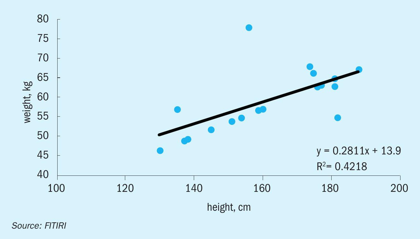
In this technique, the dependent variable is continuous, independent variable(s) can be continuous or discrete, and the nature of the regression line is linear. Linear regression establishes a relationship between a dependent variable (y) and one or more independent variables (x) using a best fit straight line (also known as regression line). It is represented by the equation where a is the intercept, b is slope of the line and e is the error term. This equation can be used to predict the value of target variable based on given predictor variable(s).

The difference between simple linear regression and multiple linear regression is that multiple linear regression has more than one independent variable, whereas simple linear regression has only one independent variable. Now the question is: how do we obtain the best line fit?

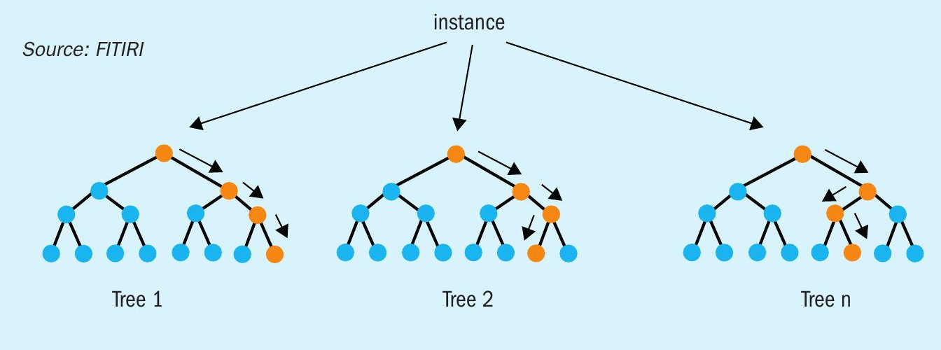
Random forest

Decision trees are great for obtaining nonlinear relationships between input features and the target variable. The inner working of a decision Tree can be thought of as a bunch of if-else conditions. It starts at the very top with one node. This node then splits into a left and right node – decision nodes. These nodes then split into their respective right and left nodes. At the end of the leaf node, the average of the observation that occurs within that area is computed. Most bottom nodes are referred to as leaves or terminal nodes.

Random forest is an ensemble of decision trees. This is to say that many trees, constructed in a certain “random” way form a random forest. Each tree is created from a different sample of rows and at each node, a different sample of features is selected for splitting. Each of the trees makes its own individual prediction. These predictions are then averaged to produce a single result. The averaging makes a random forest better than a single decision tree and hence improves its accuracy and reduces overfitting. A prediction from the random forest regressor is an average of the predictions produced by the trees in the forest.

Fig. 3: Random forest model

The random forest model is very good at handling tabular data with numerical features, or categorical features with fewer than hundreds of categories. Unlike linear models, random forests are able to capture non-linear interaction between the features and the target. The random forest model is a type of additive model that makes predictions by combining decisions from a sequence of base models. More formally we can write this class of models as:

Operational data correlations

We were able to get 30,000 readings for each parameter of the CO2 removal system. However, we got only 38 readings for the gas composition of the absorber inlet process gas, and there is no flow meter for this inlet gas. This means we cannot directly compute the amount of CO2 to be removed (absorber inlet flow x % CO2 in the inlet gas). This quantity is one the most important parameters in evaluating the CO2 removal system performance.

We therefore calculated this load in an indirect way: we used the feed natural gas flow to the primary reformer and calculated the carbon amount from natural gas analysis. Each carbon atom in the feed gas will create one molecule of CO2 in the absorber inlet, minus the small amount of CO exiting the LTS. This can be a powerful tool to determine the CO2 load into the absorber. However, the gas analysis may not be available on an hourly basis, so this can be assumed to be the same between monthly analyses without introducing too much error. Furthermore, if the calorific value of the natural gas is available, this can be used in place of the gas composition.

LTS outlet CO concentration generally tends to stay the same and changes gradually with LTS catalyst activity. If you have an LTS CO slip online analyser, that would be ideal, but even if you only have this analysis done in the lab once per month or so, it will still be acceptable; this small CO concentration does not introduce much error in the total CO2 load. We already have the feed gas flow data for every two hours and the LTS outlet analysis for CO.

The great thing about analytics is that we need to only identify the critical parameters, or their equivalent parameters and the system will correlate and find the relation. The corresponding correlation and the prediction will be as accurate as inputting the original parameter. We do not need to convert the fed gas analysis into carbon numbers and subtract the LTS CO etc, we just feed the gas analysis, feed gas flow and LTS outlet CO concentration and the model will do the rest.

In the same way, the absorber outlet CO2 slip is also critical. Absorber outlet CO2 (CO2 slip) is the main objective parameter of a CO2 removal system. Most plants have online analysers for continuous measurement. If it is not measured on a continuous basis, we can also use methanator delta T, since it will be correlated to CO2 slip for a known LTS CO slip. The methanator delta T is the sum of CO that is methanated to CH4 and CO2 that is methanted to CH4 . Both these reactions are exothermic. The predictability of the rise in temperature is very accurate as both reactions are using dry gases and the gases involved in heat rise calculation are mainly ideal gases such as H2 and N2 . We can also see this in the COORS model output showing one on one correlation to CO2 slip.

After removing high correlation variables, we got a good set of highly significant variables.

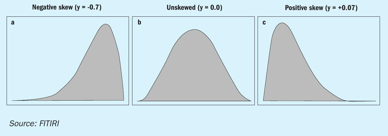
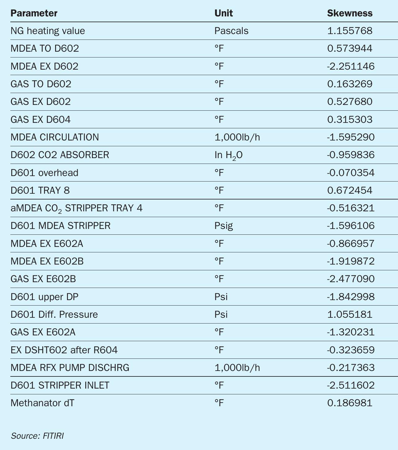
Skewness

A data is called skewed when a curve appears distorted or skewed either to the left or to the right, in a statistical distribution. In a normal distribution, the graph appears symmetrical – meaning the number of values on the left side of the mean is same as to the right side (Figure 4). Our skewness result was as shown in Table 1.

Data normalisation

During start up and shutdowns the delta T of the methanator tends to be negative or very small. Since these are not an accurate representation of the performance of the absorber and stripper and the system as a whole, dT values below 10 degrees were removed from the dataset. Also, values above 65 degrees were removed. This helped to significantly improve the accuracy of the model.

Similarly, natural gas heating value less than 37, stripper exit temperatures below 300°F, stripper inlet temperatures less than 214°F and more than 360°F were removed. This helped to create a dataset with minimal skewness and outliers.

Standard scaling was performed on the data such that its distribution will have a mean value of 0 and standard deviation of 1. Given the distribution of the data, each value in the dataset will have the sample mean value subtracted, and then divided by the standard deviation of the whole dataset.

In machine learning models, we use a portion of the data to build the model and the rest of the data to test the model. In COORS we used 75% of the data for training the model and 25% for testing the model.

Results and predictions

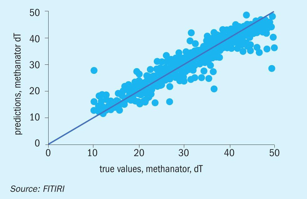
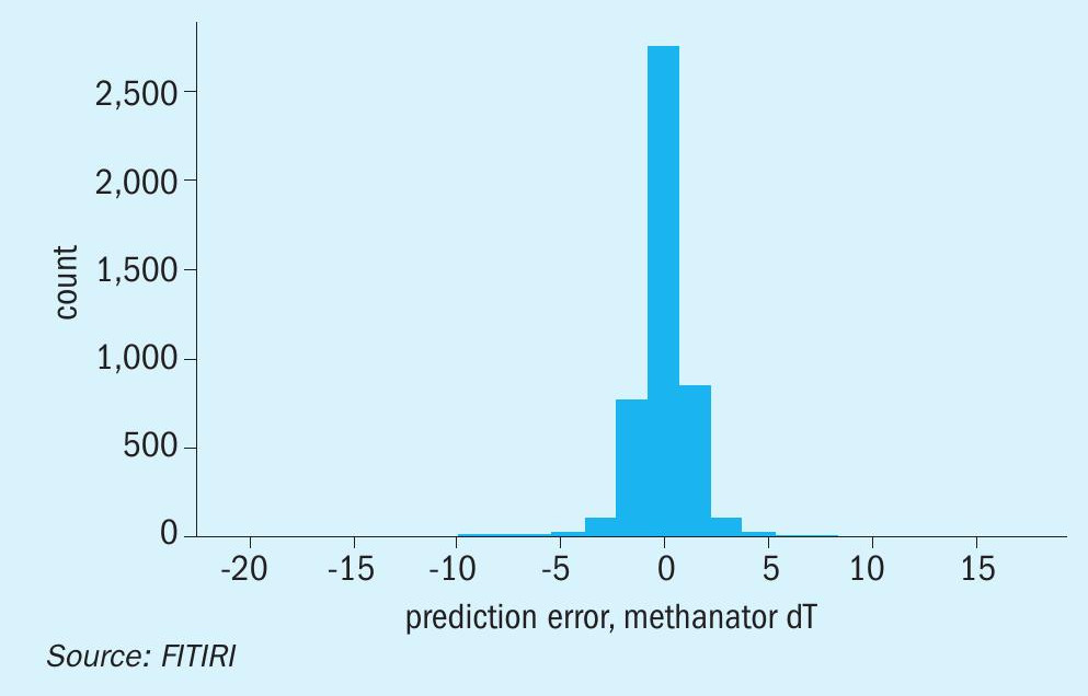
The model yielded an accuracy of 96.85 % and a mean absolute error of 0.92 degrees (Figure 5). Our prediction error provided a nice bell curve around 0 (Figure 6).

Fig. 6: Prediction error (for methanator temperature differential)

A random set of data for 15 readings were selected for prediction with the machine learning model we have built with the data provided to us. The results for the sample data gave very satisfactory results, with a mean percentage error of 1.8%.

Multiclass models also generate an independent feature importance vector for each class. Each class’s feature importance vector demonstrates which features made a class more likely or less likely. The results from this study showed that aMDEA circulation was the most important variable, with aMDEA stripper pressure in D601, gas temperature exiting D604 and aMDEA temperature exiting E602a also scoring highly.

Conclusions

We were able to predict the methanator delta T within the range of +/0.92°F. Since this is directly related to the amount of carbon dioxide coming out of the removal system, we were able to accurately identify the parameters that affect the amount of CO2 and also their impact on the system efficiency. We identified aMDEA circulation as the most critical parameter that the plant operations should keep in mind to bring down the CO2 levels in the methanator. These results were achieved through data analytics and machine learning approach rather than though traditional calculations or simulations.